Accuracy of PCA

Once, I asked James Bond where his most difficult mission took place — was it in Turkey, Mexico, or Russia?

“In Great Britain, when I was promoted to the central analytical office of MI-6,” he answered.

“Were the headquarters suddenly attacked by an army of foreign spies?”

“I would have wished for that. Instead, I had to read endless reports from other secret agents abroad and try to understand what was going on.”

“Was that so difficult?”

“Mission impossible. Imagine this: some agent informs us that State X is planning to attack the UK on a certain date with all its ground, naval and air forces. Such an important message requires verification. Another agent confirms the dreadful plans of State X but claims they intend to attack State Y, not the UK. The third agent shares with us that State Y will indeed be soon invaded, but by State Z, not State X. What would you do when receiving hundreds of such messages?”

“I would kill myself. “

James Bond carefully evaluates all available information.

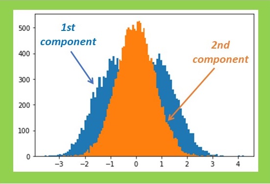
“I was on the verge of doing that. However, my older colleague advised me to relax, as he thought nobody was going to attack. We then developed a specific approach to understand the agents’ reports. You know, each agent is 100% confident in their information. However, this confidence is often subjective. We refer to this subjectivity as noise. Moreover, competing countries can intentionally fabricate and issue disinformation, which we call bias. All we need to do is collect a vast amount of data, calculate the noise (subjectivity) distribution, subtract the bias (disinformation), and extract the truth.”

“You’re suggesting that you calculate this using specific formulas? What might they look like?”

“No further comments. I can only provide you with one reference Secret Reference. If you read it carefully, you might gain an impression of how we handle big data.”

Evaluate accuracy of PCA

This conversation completely changed my understanding of how a secret service functions in reality. To delve deeper into the topic, I pursued Bond’s reference discovering an article by Noaz Nadler, a mathematician at the Weizmann Institute of Science. I thoroughly studied the article and attempted to verify its findings with some simulated spectrum-images.

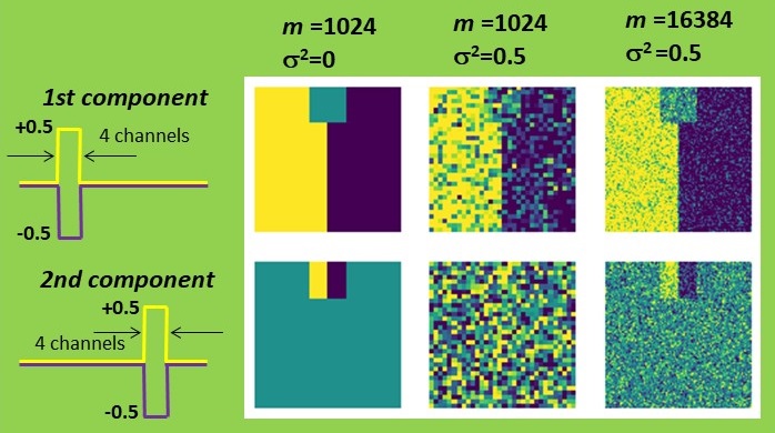
First, I constructed a simple dataset consisting of 32 by 32 pixels, each comprising 64 spectroscopic channels. The signal exhibited a rectangular shape and could be either positive or negative, resembling a characteristic line of a certain chemical element being emitted or absorbed. This signal variation is symmetric with a zero mean, simplifying the estimation process. The left half of the set was intended to represent the positive signal, while the right half represented the negative signal. One can map such a signal by summing all signal channels or by attempting to retrieve its distribution with PCA. Both methods yield identical results in the absence of noise. However, when Gaussian noise is introduced, PCA significantly outperforms simple summation. The result is still not perfect, but it appears quite reasonable.

Dataset with a simplest signal variation: positive signal at the left, negative at the right.

Now, a question arises: what is our criterion for estimating the accuracy of PCA? The simplest approach is to compare the shape of the PCA-recovered signal with the true one, which is precisely known in this case. Let’s sum the quadratic deviations over all channels and denote it as ∆2. Note that the appearance of the PCA-reconstructed maps correlates nicely with such a criterion: fewer deviations in the signal shape result in less noisy maps.

Signal profile is restored not perfectly by PCA. More its shape deviates from the true reference, more noisy are reconstructed maps.

The cited paper suggests that PCA accuracy depends on the following parameters: the number of pixels m (32×32=1024 in our case), the number of channels n (64), the variance of noise σ2, and the variance of the true, noise-free signal α2. Calculating α2 might not be straightforward. I’ll just mention that it is exactly 1 in our case. Those interested in verifying this should refer to Exercise 1 in Full Text with Codes.

The paper then demonstrates that an error in PCA reconstruction is described very simply:

Deviation of the PCA-reconstructed signal shape from the truth as a function of noise.

However, this simplicity holds true only for small σ2. The subsequent statement of the cited paper is even more instructive. When σ2 reaches a certain threshold, accuracy collapses to zero, ∆2 is undefined. There is no useful information in the dataset anymore; at least, nothing can be extracted by such a powerful method as PCA. This situation is reminiscent of James Bond’s troubles when too many contradictory reports actually provide no useful information.

The threshold for the loss of information is:

At this point, I apologize for inundating you with too many formulas. However, as you see in the modern world, even secret agents are increasingly relying on formulas rather than old-fashioned master keys in their work.

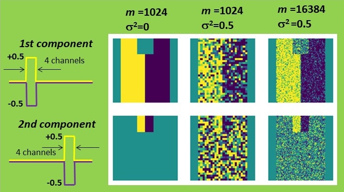
Now, back to our business! I validated the theory by altering the number of pixels m and the noise level σ2 in my dataset. In all cases, PCA accuracy improved as m increased or σ2 decreased, precisely as predicted. Moreover, when the combination of parameters reached the magic Nadler ratio (2), the maps became irretrievable.

 PCA-reconstructed maps when varying noise and number of pixels.

For those interested in further testing the Nadler model, I have prepared Exercises 2 and Exercise 3 in Full Text with Codes. The Python codes are attached. Have fun!

Comments

6 responses to “Accuracy of PCA”

  1. Ivan Rucheev Avatar
    Ivan Rucheev

    Thank you for the good example. However, I think the topic is not completely clarified. Suppose that we have an atomic lattice with two kinds of atoms, A and B. But at one cell, atom B is replaced for atom C. Assume that PCA sucessfully denoises A-B lattice but doesnot retrieve a singular atom C. The formula (1) in your post advises to increase the number of pixels to improve accuracy. But even if we scan over ten times more A-B cells, that would not help to uncover a singular C atom. This violates a common sense. Thus, I think the theory is incomplete and must be extended to the case of multicompound system and account for interaction among compounds.

    1. pavel.temdm Avatar
      pavel.temdm

      The theory is complete, just its presentation in the post is fragmentary. You are right, in multi-component sets, the things can be a bit more tricky.

      To model the situation you described, I introduced a small 8×8 pixels fragment into the 32×32 pixel set. In this fragment, quite different spectroscopy channels are activated, as if another chemical element appears or disappears. PCA is expected to detect the second principal component, which varies within this small fragment only. This is indeed the case in the noise-free case.
      Two-component dataset when the 2nd component occupies only 1/16 fraction of the whole area
      However, when noise is added, the second component suddenly becomes irretrievable. Why we observe the first component but not the second one? At the first glance, the parameters of formula (1) have not changed – added signal is of the same strength, the total number of pixel has not changed, and the noise level is same as for the first component.

      Upon careful examination, it is revealed that the noise-free data distribution alpha^2 in the second component differs drastically from that in the first one. This is because the second component counts to zero in most pixels, namely 1024-64=960 pixels. Therefore, although the signal strength is same in both components, the data variance alpha^2 in the second component would be 1024/16=16 less than that in the first one. This easy to notice if we recall that the variance is the average squared deviation from the mean (zero in this case). According to formula (2) the second component would reach the Nadler threshold at 16 times lower noise variance sigma^2 than the first component.
      The data distribution in the 2nd component is much sharper than that in the 1st one. This is because 2nd component is zero in most of the pixels
      You can verify this by examining the figure where sigma^2 of 0.5 still appears acceptable for uncovering the variation of the first component but fully suppresses extraction of the second component. This limitation cannot be overcome by scanning over the larger area. In that case, m does increase but the variance of the second component decreases proportionally.

      What would genuinely help is an increase in m through more dense scanning. The last column in the figure represents the same dataset with sampling increased four times. You can observe that both the first and second components are successfully retrieved now. While m increases by 16 times, alpha^2 remains the same as the number of pixels in the fragment increases proportionally. It is easy to confirm with formula (2) that the second component is now below the Nadler threshold.

      You can find the Python codes in Full text with codes.

  2. Ivan Rucheev Avatar
    Ivan Rucheev

    There is also so called “local PCA” to deal with such an issue. Can you comment ?

    1. pavel.temdm Avatar
      pavel.temdm

      Yes. The “local PCA” introduced by Ishizuka and Watanabe in the conference in Prague in 2014 was designed exactly for the described situation when some components are expected to be strongly spatially localised. The authors suggested to break the whole dataset on equal fragments, like a grid and perform PCA in each fragment independently.

      Let’s apply this strategy to our example and divide the set into smaller fragment. Please forgive me for cutting a bit the edges of the set, otherwise programming would be too complicated. You see from figure below that the local PCA indeed precludes the loss of the second component but makes the first component more noisy. I will try to explain why it happens.

      Two-component dataset treated by local PCA

      At small sigma^2 the accuracy of the second component extraction is not changed by local PCA. Indeed, m is decreased 16 times while alpha^2 is 16 time increased, thus formula (1) remains balanced. However, the situation is different at high sigma^2 when formula (2) should be applied. It is easy to see that the right part of (2) decreases slower with m when comparing to the left one. As a result, the larger noise level sigma^2 is needed to reach the Nadler threshold for the loss of information.

      Such strategy is however not good for the dominant first component. The local PCA does not profit from averaging over the large area and the first component is more affected by noise.

      To summarize: the local PCA can be useful however requires a great care – it improves one things while worsening the others.
      I would recommend the following:

      1. Apply it only when datasets consist of periodic fragments like atomic lattice and you have a strong suspicion that the unit cells are not identical.

      2. Set the PCA fragments approximately equal to the unit cell size. The smaller size would add more noise to the PCA results.

      3. Always compare to the PCA of the whole set.

      You can find the Python codes in Full text with codes.

  3. Jens Avatar
    Jens

    I guess your modelling accounts for noise in data. How about “subtract the bias (disinformation)”?

    1. pavel.temdm Avatar
      pavel.temdm

      Ohhh. I missed that point in the Bond’s talk. Next time I will ask. Maybe he will give me a hint.

Leave a Reply

Your email address will not be published. Required fields are marked *